Starting with the exercise we are given a dataset 'ex1data1.txt' The problem says we have to implement linear regression with one variable to predict profits for a food truck. Suppose you are the CEO of a restaurant franchise and are considering different cities for opening a new outlet. The chain already has trucks in various cities and you have data for profits and populations from the cities.

You would like to use this data to help you select which city to expand to next.

Firstly, We will import all relevant libraries and load the dataset.

#Importing necessary Libraries
import numpy as np
import pandas as pd
import matplotlib.pyplot as plt

data = pd.read_csv("ex1data1.txt")

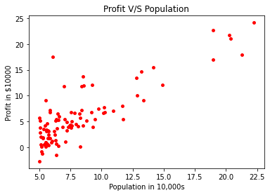
It's a good practice to visualize your data before you work on the problem so that you get a better understanding of what needs to be done and what is the relationship between the target(y) and the feature(X) variable.

feature = data["Population"]
target = data["Profit"]

plt.scatter(feature, target, c ="red", s=15)

plt.title("Profit V/S Population")
plt.xlabel("Population in 10,000s")
plt.ylabel("Profit in $10000")

Before we move on to write down the cost function J(Θ) and function for gradient descent we will perform a little manipulation on the data and convert it into NumPy array.

#Converting the data in pandas to numpy array format
X = feature.to_numpy()

#Resizing the data 
X = np.resize(X, (97,1))

#Creating an array of "1's" to append
ones = np.ones((97,1))

#Final Feature array creation
X_feature = np.append(ones,X,axis=1)

#Converting target Data into numpy array
Y = target.to_numpy()
Y_target = np.resize(Y, (97,1))

Now on to computing the cost function J(Θ)

#Cost Funtion:
def cost_function(X,theta,Y):
    """
    Take in a numpy array X,y, theta and generate the cost of using 
    theta as parameter in the model
    """
    m = X.shape[0]
    avg = (1/(2*m))

    estimate = np.square(((np.dot(X,theta))-Y))
    sqr_estimate = np.sum(estimate)
    cost = avg * sqr_estimate
    return cost

We will initialize parameters that we will be needing for Gradient Descent.

#Parameter Initialization
iterations = 1500
theta = np.zeros((2,1))
alpha = 0.01

Now we will write the Gradient Descent Algorithm:

def gradient_descent(theta,alpha,iterations,X,Y):
    """
    Take in numpy array X, y and theta and update theta by taking i gradient 
    steps
    with learning rate of alpha

    return history of theta0 and theta1 and the history of the cost of theta during each 
    iteration
    """
    m = X.shape[0]
    theta0 = np.zeros((iterations,1))
    theta1 = np.zeros((iterations,1))
    J_history = np.zeros((iterations,1))
    i = 0
    while i!=iterations:
        estimate = ((np.dot(X,theta))-Y)

        temp1 = (1/m) * np.sum(estimate)
        temp2 = (1/m) * np.sum(estimate * X)

        theta[0][0] = theta[0][0] - (alpha * temp1)
        theta0[i][0] = theta[0][0]
        theta[1][0] = theta[1][0] - (alpha * temp2)
        theta1[i][0] = theta[1][0]

        J_history[i][0] = cost_function(X,theta,Y)
        i+=1

    return J_history,theta0,theta1

Finally, we will call the function gradient_descent which will give us values of theta which we will use in our hypothesis and print it.

cost,theta1,theta2 = (gradient_descent(theta,alpha,iterations,X_feature,Y_target))
print("h(x) ={} + {}x1".format((round(theta[0,0],2)),(round(theta[1,0],2))))

The print statement will print out h(x) =-3.87 + 1.19x₁ which shows the optimized Θ values rounded off to 2 decimal places

Before we use our model to do prediction we will plot our hypothesis to get a better idea of how good our hypothesis is.

#Plotting the hypothesis
y = np.dot(X_feature,theta)
plt.scatter(feature, target, c ="red", s=15)
plt.plot(X,y)
plt.xlabel("Population in 10,000s")
plt.ylabel("Profit in $10000")
plt.title("Linear regression with one variable")

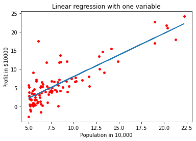
A good fit!!!!!!!😊

Now let's do some prediction:

#Doing Prediction
def predict(x,theta):
    predictions= np.dot(x,theta)
    return predictions[0]


predict1=predict(np.array([1,3.5]),theta)*10000
print("For population = 35,000, a profit of ${} is predicted".format(round(predict1,0)))

predict2=predict(np.array([1,7]),theta)*10000
print("For population = 70,000, a profit of ${} is predicted".format(round(predict2,0)))

The print statement will print out:

For population = 35,000, a profit of $4970.0 is predicted

For population = 70,000, a profit of $45512.0 is predicted

As Andrew Ng instructed in his course to visualize how cost decreases with every incrementation we will do that as well

#Checking Gradient Descent
iter = np.arange(1,iterations+1)
iter = np.resize(iter,(iterations,1))

fig, ax = plt.subplots()
ax.plot(iter, cost)

ax.set(xlabel='iteration', ylabel='cost value(J)',
       title='Checking Gradient Descent')
ax.grid()

fig.savefig("test.png")
plt.show()

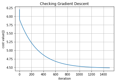
Gradient Descent seems to work fine😊.

With that we wrap up the first exercise. Hope you enjoyed reading it. Feel free to leave me any comment on any ways that I can improve my code. If you want to access the notebook for this assignment, I have uploaded the code on Github (github.com/qusaikader/Machine-Learning-Andr..).

Thanks for reading.